Expected value and variance of some stochastic processes
14 Oct 2016
As an exercise, I illustrate how expected value and variance of some stochastic processes evolve in time.
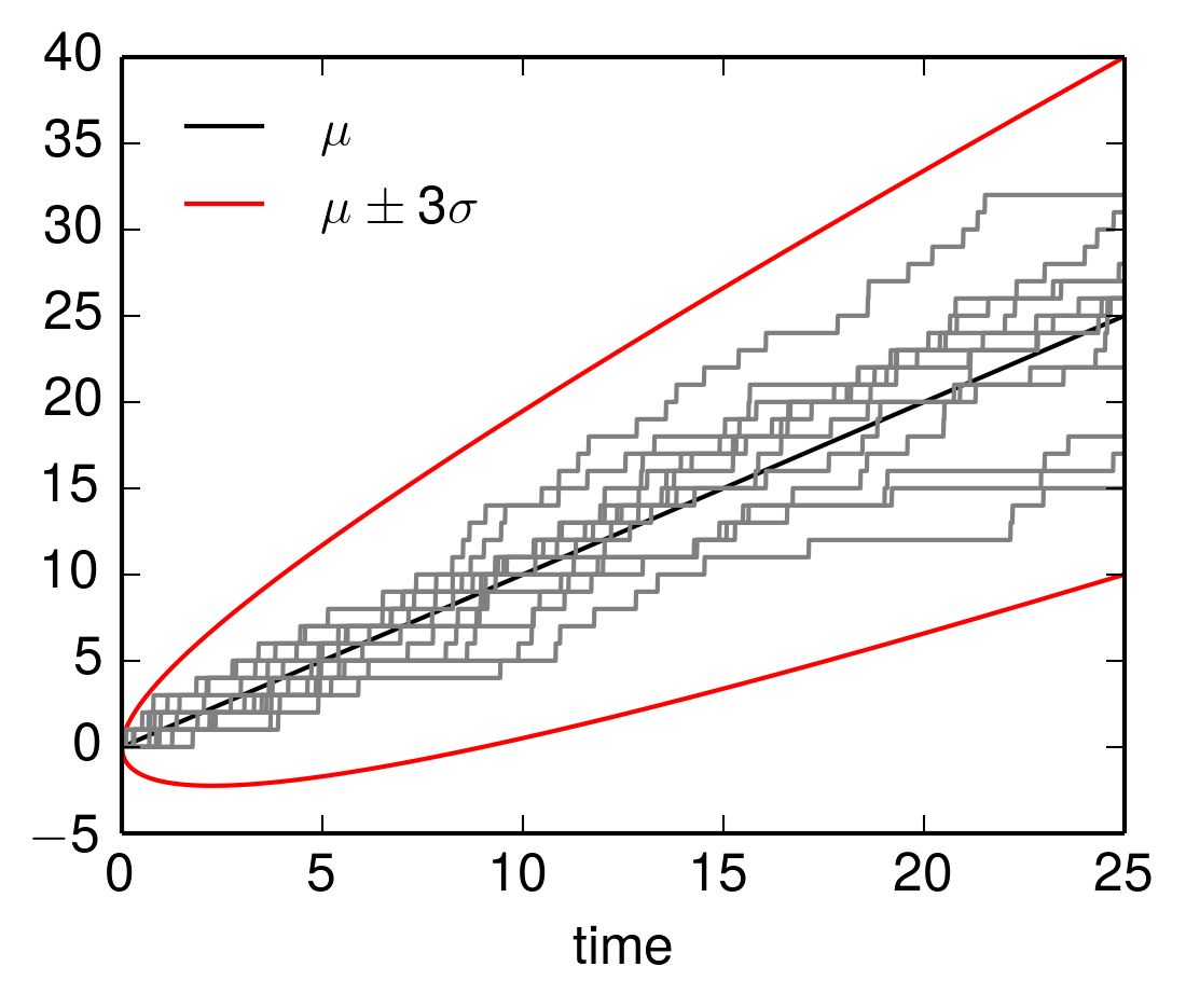
Poisson process
Let \((N_t)_{t \in \left[0,\infty\right)}\) be a Poisson process with rate \(\lambda\). Then \(\operatorname{E}(N_t) = \lambda t\) and \(\operatorname{Var}(N_t) = \lambda t\). Below several paths of a Poisson process are shown. These are well contained within \(\operatorname{E}(N_t)\) plus and minus the three time standard deviation \(3 \sigma\), where \(\sigma = \sqrt{\lambda t}\) from above.
The figure was produced by the following Python code
import numpy as np

class Poisson_process(object):

    def __init__(self, rate, dt=0.01):
        self.N = 0
        self.t = 0
        self.dt = dt
        self.rate = rate

    def sample_path(self, T, reset=None):

        path = []

        if reset != None:
            self.N = reset

        for t in np.arange(0,T,self.dt):
            k = np.random.poisson(self.rate*self.dt)
            if k>0:
                self.N+=1
            path.append(self.N)

        return path


rate = 1.
dt = 0.01
pp = Poisson_process(rate, dt=dt)
T = 25
ts = np.arange(0,T,dt)

import matplotlib as mpl
mpl.use('Agg')
import pylab as pl
from matplotlib import rc

rc('text', usetex=True)
pl.rcParams['text.latex.preamble'] = [
    r'\usepackage{tgheros}',    # helvetica font
    r'\usepackage{sansmath}',   # math-font matching helvetica
    r'\sansmath'                # actually tell tex to use it!
    r'\usepackage{siunitx}',    # micro symbols
    r'\sisetup{detect-all}',    # force siunitx to use the fonts
]


fig = pl.figure()
fig.set_size_inches(4,3)

pl.plot(ts,ts, 'k', label=r'$\mu$')

pl.plot(ts, ts+3*np.sqrt(rate*ts), 'r', lw = 1., label=r'$\mu \pm 3 \sigma$')
pl.plot(ts, ts-3*np.sqrt(rate*ts), 'r', lw = 1.)


for k in range(12):
    path = pp.sample_path(T, reset=0)
    pl.plot(ts, path, 'gray')

pl.legend(loc='upper left', frameon=False, prop={'size':12})

pl.xlabel('time')

pl.savefig("pp_sample.png", dpi=300, bbox_inches='tight')
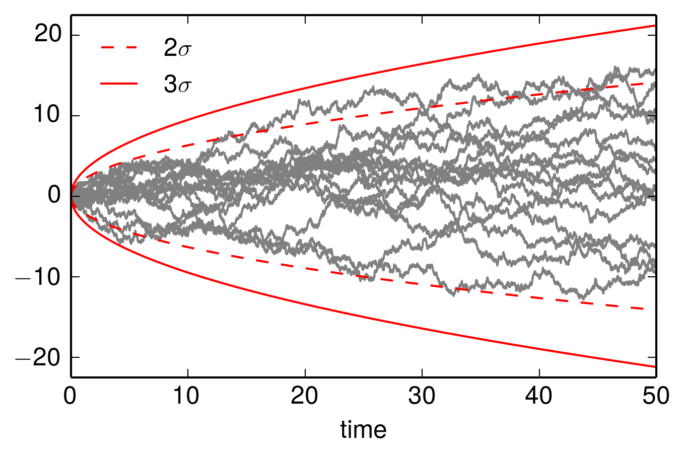
Wiener process
Let \((X_t)_{t \in \left[0, \infty\right)}\) be a Wiener process. It is \(\operatorname{E}(X_t) = 0\) and \(\operatorname{Var}(X_t) = t\). Below 15 sampled paths of the Wiener process are shown. It's trace are well contained within \(2 \sigma\) or \(3 \sigma\), where \(\sigma = \sqrt{t}\) is the standard deviation.
The figure was generated by the following Python code
import numpy as np

class Wiener_process(object):

    def __init__(self, dt=0.01):
        self.X = 0
        self.t = 0
        self.dt = dt

    def sample_path(self, T, reset=None):

        path = []

        if reset != None:
            self.X = reset

        for t in np.arange(0,T,self.dt):
            x = np.random.normal(0,np.sqrt(self.dt))
            self.X+=x
            path.append(self.X)

        return path


dt = 0.01
wp = Wiener_process(dt=dt)
T = 50
ts = np.arange(0,T,dt)


import matplotlib as mpl
mpl.use('Agg')
import pylab as pl
from matplotlib import rc

rc('text', usetex=True)
pl.rcParams['text.latex.preamble'] = [
    r'\usepackage{tgheros}',    # helvetica font
    r'\usepackage{sansmath}',   # math-font matching helvetica
    r'\sansmath'                # actually tell tex to use it!
    r'\usepackage{siunitx}',    # micro symbols
    r'\sisetup{detect-all}',    # force siunitx to use the fonts
]


fig = pl.figure()
fig.set_size_inches(5,3)

for k in range(15):
    path = wp.sample_path(T, reset=0)
    pl.plot(ts, path, 'gray')

pl.plot(ts, 2*np.sqrt(ts), 'r', linestyle='dashed', lw=1., label=r'$2 \sigma$')
pl.plot(ts, -2*np.sqrt(ts), 'r', linestyle='dashed', lw=1.)

pl.plot(ts, 3*np.sqrt(ts), 'r', lw = 1., label=r'$3 \sigma$')
pl.plot(ts, -3*np.sqrt(ts), 'r', lw = 1.)

pl.ylim(-22.5,22.5)

pl.legend(loc='upper left', frameon=False, prop={'size':12})

pl.xlabel('time')

pl.savefig("wp_sample.png", dpi=300, bbox_inches='tight')
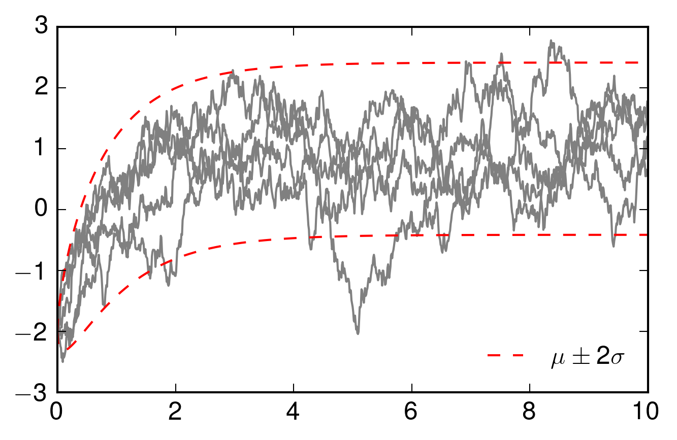
Ornstein-Uhlenbeck process
Let \((X_t)_{t \in [0,\infty)}\) be an Ornstein-Uhlenbeck process, that is a process defined by the stochastic differential equation
with \(X_0 = a\). The expected of value this process is
and the variance is
import numpy as np

class OU_process(object):

    def __init__(self,X_0, mu, theta, sigma, dt=0.01):
        self.X = X_0
        self.dt = dt

        self.mu = mu
        self.theta = theta
        self.sigma = sigma

        self.setup()


    def setup(self):
        self.emdt = np.exp(-self.theta*self.dt)
        self.a = np.sqrt(self.sigma**2/(2*self.theta) *
                         (1 - np.exp(-2*self.theta*self.dt)))


    def step(self):
        X_dt = self.X*self.emdt+self.mu*(1 - self.emdt) + \
                 self.a*np.random.normal()
        self.X = X_dt


    def path(self, T, reset=None):

        if reset != None:
            self.X = reset

        path = []
        for t in np.arange(0,T,self.dt):
            path.append(self.X)
            self.step()
        return path


dt = 0.01
X_0 = -2
mu = 1.
theta = 1.
sigma = 1.

OU = OU_process(X_0, mu, theta, sigma, dt)

import matplotlib as mpl
mpl.use('Agg')
import pylab as pl
from matplotlib import rc

rc('text', usetex=True)
pl.rcParams['text.latex.preamble'] = [
    r'\usepackage{tgheros}',    # helvetica font
    r'\usepackage{sansmath}',   # math-font matching helvetica
    r'\sansmath'                # actually tell tex to use it!
    r'\usepackage{siunitx}',    # micro symbols
    r'\sisetup{detect-all}',    # force siunitx to use the fonts
]


T = 10
ts = np.arange(0,T,dt)

mean = np.array([X_0*np.exp(-theta*t) + \
                 mu*(1-np.exp(-theta*t)) for t in ts])
var = np.array([sigma**2/(2*theta)* \
                  (1-np.exp(-2*theta*t)) for t in ts])

fig = pl.figure()
fig.set_size_inches(5,3)

for k in range(5):
    path = OU.path(T, reset=X_0)
    pl.plot(ts, path, 'gray')

pl.plot(ts, mean+2*np.sqrt(var), 'r', linestyle='dashed',
        lw=1., label=r'$\mu \pm 2 \sigma$')
pl.plot(ts, mean-2*np.sqrt(var), 'r', linestyle='dashed',
         lw=1.)

pl.ylim(-3,3)

pl.legend(loc='lower right', frameon=False, prop={'size':12})

pl.savefig("ou_sample.png", dpi=300, bbox_inches='tight')