Comparing the Euler, Midpoint and Runge-Kutta method

25 Jan 2012

To find an approximate solution to the initial value problem

$$ \begin{align} y'(t) &= f(t,y(t)), \\ y(t_0) &= y_0 \end{align} $$

we compare three different methods: The Euler method, the Midpoint method and Runge-Kutta method. The accuracy of the solutions we obtain through the
different methods depend on the given step size.

Let always $e$, $m$ and $r$ denote the step sizes of Euler, Midpoint and Runge-Kutta method respectively.

In the Euler method the value $y_n+1$ of $y$ at the point $t_n+1 = t_n + e$ is is given by the first two of the taylor expansion of $y$ at $t_n$, that is

\[ y_n+1 = y_n + e\,f(t_n,y(t_n)). \]

In the Midpoint method we have $t_n+1 = t_n + m$ and

\[y_n+1 = y_n + m f\left(t_n + \frac{m}{2}, y_n + \frac{m}{2} f(t_n,y_n)\right).\]

Note, that here we have to eveluate the function $f$ twice to obtain our next value $y_n+1$, whereas when using Euler method we only needed to do this once.

Lastly the Runge-Kutta method (of fourth order) is a further refinement of the methods above, where we now have $t_n+1 = t_n + r$ and

\[y_n+1 = y_n + \frac{1}{6}(k_1 + 2k_2 + 2k_3 + k_4)\]

where the calculation of the coefficients $k_1, k_2, k_3, k_4$ requires an independent evaluation of $f$ each.

Thus the Runge-Kutta needs four steps of calculation to get the next value $y_n+1$.

When comparing the three methods, one should therefore choose the stepsizes accordingly, that is in such a way that

\[4e = 2m = r\]

holds.

A justified question is to ask wether the midpoint method yields better results than the Euler method with half the step size at all. I wrote a script to investigate that question. Here are some examples, for which I compared the three methods:

Consider $y'(t) = -2t\,y(t)$ with initial value $y(0) = 1$. We easily verify that $y(t) = \exp(-t^2)$ is an exact solution to the problem. Calculating the solutions with three different methods I got the diagram

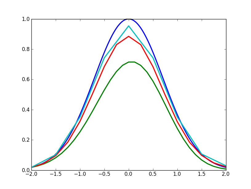Here the graphs show the exact solution and solutions obtained with the Runge-Kutta method, the midpoint method and the Euler method.

The step sizes chosen are $r=0.5$, $m=0.25$ and $e = 0.125$, thus fullfilling our requirement at them for the methods to be comparable.

We see, that while the Euler method does yield the smoothest curve it yields the worst result. Here, the way in which the next value $y_{n+1}$ is determined is inaccurate compared to the other two methods and since $y_{n+2}$ depends on $y_{n+1}$, this error progresses in the calculation to eventually yield only a very vague approximation.

Here is another example:

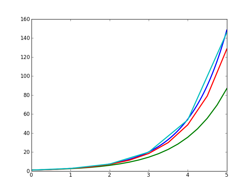To solve $y'(t) = y(t)$, which of course has the exact solution $y(t) = \exp(t)$, the following step sizes where chosen: \[r=1, m=0.5 \,\, \textrm{and} \,\, e = 0.25\]

What I wanted to show are two examples in which the Runge-Kutta method yields better results than the Midpoint and Euler method, although for those step sizes are chosen accordingly smaller to have a comparable effort in computation.

Please keep in mind that I did this small project mostly in an effort to learn Python. Take what you will out of my descriptions here, but take caution in any case.

Here's the code that I used. Careful, it's a mess as I'm programming Python for only a very short time!

import matplotlib.pyplot as plt
import numpy as np

"""
def dy_dt(t,y_t):
        return y_t

def y(t):
        return np.exp(t)

t_range = (0,5)

k=1.0
initial_value_pair = (t_range[0],np.exp(t_range[0]))
euler_stepsize = k/4
midpoint_stepsize = k/2
runge_kutta_stepsize = k
"""

def dy_dt(t,y_t):
        return -2*t*y_t

def y(t):
        return np.exp(-t**2)

t_range = (-2,2)

initial_value_pair = (t_range[0],np.exp(-t_range[0]**2))
euler_stepsize = 0.125
midpoint_stepsize = 0.25
runge_kutta_stepsize = 0.5



figure = plt.figure(facecolor="white")


#Draw exact solution

exact_t_range = np.arange(t_range[0],t_range[1],(t_range[1]-t_range[0])/10000.)
exact_y_vals = y(exact_t_range)
plt.plot(exact_t_range,exact_y_vals, linewidth=2.5)  


#Draw Euler solution

h=euler_stepsize
euler_t_range = np.arange(t_range[0],t_range[1]+h/1000., h)
euler_y_vals = np.array([initial_value_pair[1]])

for k in euler_t_range:
        if k == t_range[0]:
                continue
        else:
                next_entry = euler_y_vals[-1] + h*dy_dt(k-h,euler_y_vals[-1])
                euler_y_vals = np.append (euler_y_vals, next_entry)

plt.plot(euler_t_range,euler_y_vals, linewidth=2.5)


#Draw Midpoint solution

h=midpoint_stepsize
midpoint_t_range=np.arange(t_range[0],t_range[1]+h/1000.,h)
midpoint_y_vals=np.array([initial_value_pair[1]])

for k in midpoint_t_range:
        if k == t_range[0]:
                continue
        else:
                next_entry = midpoint_y_vals[-1] + h*dy_dt(k-h+h/2,midpoint_y_vals[-1] + h/2*dy_dt(k-h,midpoint_y_vals[-1]))
                midpoint_y_vals = np.append(midpoint_y_vals, next_entry)

plt.plot(midpoint_t_range, midpoint_y_vals, linewidth=2.5)


#Draw Runge-Kutta solution

h=runge_kutta_stepsize
rk_t_range = np.arange(t_range[0],t_range[1]+h/1000.,h)
rk_y_vals = np.array([initial_value_pair[1]])

for k in rk_t_range:
        if k==t_range[0]:
                continue
        else:
                k_1 = dy_dt(k-h,rk_y_vals[-1])
                k_2 = dy_dt(k-h + h/2, rk_y_vals[-1] + h/2*k_1)
                k_3 = dy_dt(k-h + h/2, rk_y_vals[-1] + h/2*k_2)
                k_4 = dy_dt(k-h + h, rk_y_vals[-1] + h*k_3)
                next_entry = rk_y_vals[-1] + 1./6*h*(k_1 + 2*k_2 + 2*k_3 + k_4)
                rk_y_vals = np.append(rk_y_vals, next_entry)

plt.plot(rk_t_range, rk_y_vals, linewidth=2.5)

plt.show()

3 Diagrams per Page

About

Comparing the Euler, Midpoint and Runge-Kutta method